Final Project
Author: Pat Dotson
Objective Hierarchies Mathematical Representation
Variables and Attributes Testing & Validation
Influence Diagram Implementation and Use
Objective
Hierarchies
|
The objective of this exercise is to determine the maximum profitability of lot sales for Pat Dotson Builder, Inc. In order to determine the maximum profit, forecasting, simulation, and optimization will be utilized.
Time Series
Forecasting:
The objective of time series forecasting and regression on historical data is to determine the firm’s demand for its products. Time series regression is a forecasting method that involves extrapolating historical data in order to create a basis for decision-making in the future. Extrapolation methods are quantitative methods that use past data of a time series variable to forecast future values of the variable. It looks for trends and seasonality in the data and builds a formula that can be used to predict values. Time series forecasts are helpful in business for predicting consumer demand, projecting expenditures, and estimating future revenues. Regression analysis is the study of relationships between variables to establish a mathematical model to predict dependent variable, such as demand, by substituting value(s) of independent variable(s).
For this exercise, the analysis enables us to forecast the next four periods for the variables average demand, average price, and average advertising and create an equation that ultimately predicts normalized share of market demand to assist in manufacturing and financial decisions of the organization. CB Predictor will be used to run the time series forecast and Excel will be used to run the regression.
Simulation:
The objective of this analysis is determining the average cost required to develop each lot using Monte Carlo Simulation. Monte Carlo Simulation is a mathematical technique for numerically solving differential equations. Monte Carlo Simulation is used to solve a problem that requires one or more statistics of a probability distribution be calculated. The Monte Carlo Simulation calculates multiple scenarios of a model by repeatedly sampling values from the probability distributions for the uncertain variables and using those values. The cost of the developed lot provides a necessary component for a residential developer. Using Monte Carlo Simulation, the residential developer will know within a certain probability level, the expected average cost of each lot developed.
Optimization:
The objective of this exercise is to maximize firm profit using the correct mix of product pricing, advertising, production cost, and production units. This model will consider all of the components listed above to determine the maximizing profit level. In order to use optimization, critical criteria must be entered into the solver equation, (using excel) to find the optimal level. Taking all of the criteria and constraints into consideration, the solver will determine the optimal level.
This objective hierarchy is a graphical representation of the internal factors that drive the business model to profitability.

Variables
& Attributes
|
|
Variable |
How Measured |
Related to |
|
Time Series Forecasting – Average Firm Demand x Normalized Share of
Market |
||
|
Period |
In numerical order |
None |
|
Season |
Quarter of year (1, 2, 3, 4) |
Time of year |
|
Average Demand |
Units demanded |
Total demand divided by the number of firms in industry. Dependent on economy, industry, and competitive forces. |
|
Average Price |
Price in dollars |
Total sales divided by units sold. Dependent on economy, industry, and competitive forces. |
|
Average Advertising |
Dollars spent |
Total advertising expenditures divided by number of firms in industry. Dependent on economy, industry, and competitive forces. |
|
Average Advertising 1 |
Dollars spent |
Total advertising expenditures last year divided by number of firms in industry. Dependent on economy, industry, and competitive forces. |
|
Average Advertising 2 |
Dollars spent |
Total advertising expenditures two years ago divided by number of firms in industry. Dependent on economy, industry, and competitive forces. |
Regression Analysis |
||
|
Quarter |
1, 2, 3, 4 |
|
|
Firm |
Number |
Firm identifier |
|
NSOM |
Ratio: share of market |
Normalized share of market, measure of demand, determined by quality, reputation, advertising, research and advertising, and other factors. |
|
Prel |
Ratio: relative price |
Price divided by average price of industry for the quarter indicated. |
|
Arel |
Ratio: relative advertising expenditures |
Total advertising expenditures divided by average advertising expenditures of industry for the quarter indicated. |
|
NSOM1 |
Ratio: share of market |
Normalized share of market for last quarter. See NSOM. |
|
Arel1 |
Ratio: relative advertising expenditures |
Total advertising expenditures of previous quarter divided by average advertising expenditures of industry for the previous quarter. |
|
Arel2 |
Ratio: relative advertising expenditures |
Total advertising expenditures of two quarters previous divided by average advertising expenditures of industry for the two quarters previous. |
|
Forecasting
Variables: |
||
|
Activity |
Description |
All of the activities required to develop a lot from raw
land |
|
Min – Minimum Cost |
Dollars |
The minimum expected cost for each activity. Expected to
be 85% less than most likely. |
|
Most Likely Cost |
Dollars |
The expected cost for each activity. The cost is
determined based on competitive bid or intuition based on experience. |
|
Max – Maximum Cost |
Dollars |
The maximum expected cost for each activity. Expected to
be no more than 40% of the most likely cost. |
|
Implied Mean |
Dollars |
Results for triangular distribution |
|
Cost |
Dollars |
Triangular distribution. Use RISKPERT function in @ risk
software to determine. |
|
Cost + |
Dollars |
Adds one dollar to each activity to determine whether or
not this activity is critical to the overall cost of the lot. |
|
Index of activity to increase lot cost |
Numeric |
Use RISKSIM function in @risk software to run the
simulation for each activity. |
|
Optimization
Variables: |
||
|
|
Dollars |
Price of each lot expected to be sold in a particular
period. Price is a constraint on solver, whereas lot price can not dip below
$32,000. Solver will determine optimal level. |
|
Average |
Dollars |
Expenditure expected for each lot. Solver will determine
optimal level of advertising. |
|
Firm Demand |
Units |
Units to be sold in this period. Company can only produce
350 units in this period, creating a constraint on excel solver. Solver will determine
the optimal level. |
|
|
Dollars |
|
|
Operating Margin |
Percentage |
The cost of capital for Pat Dotson Builder is 12%; therefore, in order to create positive shareholder wealth, operating margin must exceed 12% or the cost of capital. If the operating margin is less than 12%, then shareholder wealth will be diminished. |
Influence
Diagram
|
This influence diagram is a graphical representation of the endogenous and exogenous factors that interface with each other to create demand for a product.

Mathematical
Representation
|
Time Series Forecast:
Average Firm Demand:
In order to develop a mathematical model to predict firm demand, two regressions need to be run, time series and least squares regression. The summary of the results of the time series forecast (run in CB Predictor) are as follows:
|
Methods |
Rank |
RMSE |
MAD |
MAPE |
Durbin-Watson |
Theil's U |
Periods |
Alpha |
Beta |
Gamma |
|
Double
Exponential Smoothing |
7 |
55.972 |
48.275 |
25.086 |
1.488 |
0.98 |
|
0.429 |
0.151 |
|
|
Double
Moving Average |
8 |
64.442 |
58.19 |
27.46 |
1.259 |
0.849 |
5 |
|
|
|
|
Holt-Winters'
Additive |
3 |
34.876 |
29.346 |
16.517 |
1.26 |
0.674 |
|
0.093 |
0.044 |
0.001 |
|
Holt-Winters' Multiplicative |
1 |
32.09 |
23.687 |
13.892 |
1.445 |
0.587 |
|
0.19 |
0.001 |
0.001 |
|
Seasonal
Additive |
4 |
38.243 |
32.07 |
17.913 |
1.817 |
0.748 |
|
0.802 |
|
0.001 |
|
Seasonal
Multiplicative |
2 |
34.619 |
26.921 |
14.596 |
1.693 |
0.652 |
|
0.565 |
|
0.001 |
|
Single
Exponential Smoothing |
5 |
51.555 |
44.483 |
22.263 |
1.565 |
0.875 |
|
0.395 |
|
|
|
Single
Moving Average |
6 |
54.551 |
49.569 |
23.975 |
1.279 |
0.836 |
4 |
|
|
|
CB Predictor determined that the Holt-Winters’ Multiplicative method was the best method for completing this time series forecast because it had the lowest Root Mean Square Error (RMSE), lowest Mean Absolute Deviation (MAD), and Mean Absolute Percentage Error (MAPE). Holt-Winters’ Multiplicative method accounts for the level and trends, as well as seasonality.
Level of the Series: Lt
= α*Yt/St-M + (1-α)(Lt-1 + Tt-1)
Trend: Tt = β(Lt - Lt-1) + (1 - β)Tt-1
Seasonality: St = γ* Yt/Lt + (1-γ) St-M
Forecast of Yt+k Ft+k = (Lt + kTt)St+k-M
M = number of seasons 4
k is the period ahead 3 months
Forecast:
|
Date |
Lower 5% |
Forecast |
Upper 95% |
|
25 |
294 |
350 |
405 |
|
26 |
270 |
328 |
386 |
|
27 |
219 |
280 |
341 |
|
28 |
217 |
282 |
346 |
Regression:
After completing this time series regression, the residuals are then used in a least squares regression against the other variables in the AFD model. This exercise found that the only variables that were significant in the prediction were average advertising and average price.
|
Regression Statistics |
|
|
Multiple
R |
0.918707 |
|
|
0.844023 |
|
Adjusted |
0.827604 |
|
Standard
Error |
13.45969 |
|
Observations |
22 |
|
ANOVA |
|
|
|
|
|
|
|
df |
SS |
MS |
F |
Significance F |
|
Regression |
2 |
18625.91 |
9312.957 |
51.40643 |
2.15811E-08 |
|
Residual |
19 |
3442.102 |
181.1633 |
|
|
|
Total |
21 |
22068.02 |
|
|
|
|
|
Coefficients |
Standard Error |
t Stat |
P-value |
Lower 95% |
Upper 95% |
Lower 95.0% |
Upper 95.0% |
|
Intercept |
1806.068277 |
227.6756445 |
7.932637 |
1.9E-07 |
1329.537529 |
2282.59903 |
1329.53753 |
2282.59903 |
|
Avg_Price |
-0.04913017 |
0.005950008 |
-8.25716 |
1.04E-07 |
-0.061583683 |
-0.03667666 |
-0.06158368 |
-0.0366767 |
|
Avg_Adv |
0.034696571 |
0.013187465 |
2.631027 |
0.016457 |
0.007094881 |
0.06229826 |
0.00709488 |
0.06229826 |
Models:
Level of the Series: Lt
= 0.19*Yt/St-M + (1-0.19)(Lt-1 + Tt-1)
Trend: Tt = 0.001(Lt - Lt-1) + (1 – 0.001)Tt-1
Seasonality: St = 0.001* Yt/Lt + (1-0.001) St-M
Forecast of Yt+k Ft+k = (Lt + kTt)St+k-M
Residual: 1806.07 + (0.049)Avg_Price + 0.0347Avg_Adv
Complete Model: Ft+k = (Lt + kTt)St+k-M + 1806.07 + (0.049)Avg_Price + 0.0347Avg_Adv
Normalized Share of
Market:
In order to predict the normalized share of the market, a least squares regression was run on the nsom spreadsheet data. All variables were found significant, here are the results:
|
Regression Statistics |
|
|
Multiple
R |
0.989143 |
|
|
0.978405 |
|
Adjusted |
0.977784 |
|
Standard
Error |
0.040064 |
|
Observations |
180 |
|
ANOVA |
|
|
|
|
|
|
|
df |
SS |
MS |
F |
Significance F |
|
Regression |
5 |
12.65383 |
2.530766 |
1576.66 |
7.4159E-143 |
|
Residual |
174 |
0.279295 |
0.001605 |
|
|
|
Total |
179 |
12.93312 |
|
|
|
|
|
Coefficients |
Standard Error |
t Stat |
P-value |
Lower 95% |
Upper 95% |
Lower 95.0% |
Upper 95.0% |
|
Intercept |
16.516 |
0.31777775 |
51.9764 |
6.51E-108 |
15.88975 |
17.144142 |
15.8897525 |
17.144142 |
|
Prel |
-17.061 |
0.31927463 |
-53.4384 |
6.92E-110 |
-17.6916 |
-16.431365 |
-17.691663 |
-16.431365 |
|
Arel |
0.7440 |
0.0194598 |
38.2346 |
1.369E-86 |
0.70563 |
0.78244573 |
0.7056305 |
0.78244573 |
|
NSOM1 |
0.4493 |
0.01351132 |
33.2581 |
2.569E-77 |
0.42269 |
0.47602904 |
0.42269473 |
0.47602904 |
|
Arel1 |
0.26290 |
0.02164047 |
12.1486 |
5.495E-25 |
0.22018 |
0.30561305 |
0.22018989 |
0.30561305 |
|
Arel2 |
0.08574 |
0.02101009 |
4.08133 |
6.813E-05 |
0.04428 |
0.12721674 |
0.04428191 |
0.12721674 |
Residual Model:
NSOM
= 16.516 + (17.061)Prel + 0.7440Arel + 0.4493NSOM1 + 0.2629Arel1 + 0.08574Arel2
Using the models from the time series forecasting, least squares regression on the AFD residuals, and the least squares regression on the NSOM data, we can create a DSS interface that provides the user the needed data for business decisions. A screenshot of this interface is below:
Forecasting:
Forecasting’s mathematical calculations were computed using @risk software in an excel spread sheet.
Results: Output Snapshot
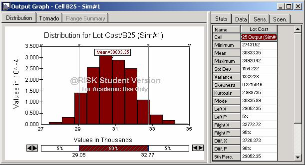
The above screen shot is one simulation, is the histogram created using @risk. The above chart shows that the cost of each lot will cost between $28,980 and 32,840 with a 90% confidence level. This means that 90% of the time the lot cost will fall within this range. The mean cost per lot is $30,833. this is the lot cost that is used to calculate the profit for the firm.
The simulation was run with 1,000 iterations and 9 simulations. One simulation was run for each activity in the cost structure of a lot. For each simulation, the mean lot cost was equal to $30,833.
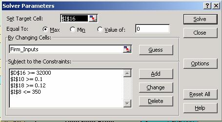
Optimization:
Solver will change this variable unit it finds the lot price
that maximizes profit.
Average
Solver will change this variable to find the advertising level that maximizes profit. This input variable is flexible and can be as little as zero with no upper limit.
Firm Demand
Average Firm demand is calculated using time forecasting and regression calculations. The user can change the current input variables to see the possible impact. Solver will take the inputs from these calculations in determining firm demand. Firm demand is constrained at 350 units. The firm can only produce a maximum of 350 units, therefore any units demanded above 350 could not be produced.
Operating Profit
Profit = (Firm Demand x
Operating Margin
Operating Margin for the company must be at least 12%. In
solver, a 12% operating margin is a constraint to find the optimal operating
profit.
Market Share
Pat Dotson Builder’s strategy is to maintain a market share of 10%. Market share of 10% is a constraint to find the optimal operating profit.
Solver:
Interface for DSS:
|
Pat Dotson Builder, Inc.-
Development DSS |
||||||||
|
Inputs |
Outputs |
|||||||
|
|
|
|
|
|
|
|
|
|
|
|
Macro |
|
|
|
|
Average
Firm Demand |
205 |
|
|
|
Period |
27 |
|
|
|
|||
|
|
Number of
Firms |
10 |
|
|
|
Share
of Market |
1.71 |
|
|
|
|
|
|
|
|
|
|
|
|
|
Industry
Inputs |
|
|
|
|
Firm
Demand |
350 |
|
|
|
Avg.
Price |
39,000 |
|
|
|
|||
|
|
Avg.
Advertising |
1,000 |
|
|
|
Market
Share |
17.07% |
|
|
|
Avg. Advertising
(t-1) |
990 |
|
|
|
|
|
|
|
|
|
|
|
|
|
|
$
13,077,326 |
|
|
|
|
|
|
|
|
|
|
|
|
|
|
|
|
|
|
|
$
11,117,521 |
|
|
|
Firm
Inputs |
|
|
|
|
|
|
|
|
|
Price |
|
|
|
Operating
Profit |
$
1,959,805 |
|
|
|
|
Advertising |
931 |
|
|
|
|
|
|
|
|
Share of
Market - (t-1) |
101.75% |
|
|
|
Operating
Margin |
14.99% |
|
|
|
Relative
Advertising - (t-1) |
122.33% |
|
|
|
|
|
|
|
|
Relative
Advertising - (t-2) |
75.30% |
|
|
|
|
|
|
|
|
|
|
|
|
|
|
|
|
The above interface is the sheet that the user will see and have the ability to change. Only the cells that are inputs in the current period are able to change. Historical and calculated values are unable to be changed by the user.
Testing
& Validation
|
To test the model, and to view the behind the scenes calculations and regression results, go to the following link:
This model is designed to calculate the outputs for the four periods following the end of the historical data (25, 26, 27, and 28.) If periods higher than these are input, the user will get an error message and no data in the output section. This interface allows the user to change many inputs to see the effect on AFD, NSOM, Firm Demand, Market Share, and Firm Revenue. These inputs include number of firms (cannot be less than 2), industry inputs (these change with new historical data and firms entering and exiting the industry), and firm inputs such as price and expenditures. The industry inputs cannot be controlled by individual firms, but the firm inputs can be controlled and are used in the model to evaluate expected outputs. These outputs help managers make decisions about these inputs.
Implementation
& Use
|
This model could be used in a much larger model that incorporates the firm’s proforma financial statements and manufacturing data. By changing the inputs, the user could see not only the outcome of demand, but also what affect this would have on the firm’s financial statements. Also, a manufacturing module could be linked to the DSS that provided data on capacity and costs.
Many reports could be written to use with this system, including proforma financial statements, demand forecasts, recommended advertising and research and development expenditures and cost data. Analyses could be conducted to answer any questions about how much to spend on advertising and expenditures, what to price the product to get the desired market share and resulting revenue. This would be an example of goal seeking where the desired output is entered and the variables are found that create that result. This module could also be used to evaluate scenarios such as good economy or recession. The module could also be used to run what-if analyses, for example to see the result in a big increase in advertising executives salaries that cause advertising expenditures to increase for the same amount of advertising.