Optimization
Chandler Oil
Company
Authors:
Pat Dotson
Situation Description and Overall Objective Mathematical Representation
Variables and Measures Development of Spreadsheet Model and Results
Influence Diagram DSS Guidelines
Situation Description and Overall Objective
|
The objective of this exercise is to maximize firm profit using the correct mix of products. The model will only consider the revenue to determine the optimal level. Typically cost would be consider in most situation, for simplicity to show the use of excel solver, advertising will be the only cost component considered. In order to determine the optimal product mix, the following factors need to be considered:
· Market demand for each type of product the company produces.
· Firm demand for each type of product the firm produces.
· Firm resources available to produce each type of product.
· Advertising cost for each type of product.
· Quality level required to produce each type of product.
For this example, the company, Chandler Oil, produces only two types of products. The two products produced, gasoline and heating oil, require the same type of raw material to produce the end product. The only difference for the two products is the mix required to produce the end product. To produce the gasoline and heating oil, two types of crude oil are required, crude oil 1 and crude oil 2. Crude oil one is of higher quality and cost more than crude oil two. Gasoline requires a higher quality than does heating oil leading to a higher average cost per barrel of gasoline . Since gasoline requires a higher quality standard than heating oil, the company can produce less gasoline than heating oil with the raw materials available. The model will take into account all of the different factors list above, using solver within excel, to determine the optimal level of production to maximize company profit.
Variables & Measures
|
|
Variable |
How Measured |
Description |
|
Time Series Forecasting |
||
|
Crude Oil One |
Barrels |
5000 barrels available for production. This limited level of supply will put a production constraint on the company. |
|
Crude Oil One |
Quality Level |
10 quality points per barrel creates a constraint for the company. |
|
Crude Oil Two |
Barrels |
10,000 barrels available for production. This limited
level of supply will put a production constraint on the company. |
|
Crude Oil Two |
Quality |
5 quality points per barrel creates a constraint for the
company. |
|
Gasoline – Selling Price |
Dollars per Barrel |
Selling Price determined by market demand using a supply
demand curve. |
|
Gasoline |
Quality Points |
Must exceed a quality level of 8 points |
|
Heating Oil – Selling Price |
Dollars per Barrel |
Selling Price determined by market demand using a supply
demand curve. |
|
Heating Oil |
Quality Points |
Must exceed a quality level of 6 points |
|
Advertising Gasoline |
Dollars per Barrel |
Advertising cost per barrel of gasoline is set for this example at $0.20 per barrel. |
|
Advertising Heating Oil |
Dollars per Barrel |
Advertising cost per barrel of heating oil is set for this
example at $0.10 per barrel. |
|
Total Revenue |
Dollars |
Revenue is determined by multiplying the number of barrels of each product sold by its selling price. |
|
Total Advertising Cost |
Dollars |
Advertising expenditures is determined by multiplying the number of barrels sold for each product sold by its advertising cost per barrel. This model assumes that every barrel of product produced is sold leaving no product in inventory. |
|
Heating Oil Produced |
Barrels |
This variable will be calculated using solver to determine the maximum profit level. |
|
Gasoline Produced |
Barrels |
This variable
will be calculated using solver to determine the maximum profit level. |
|
Company Profit |
Dollars |
This is the objective of the exercise. Using solver and all of the inputs, solver will determine the optimal level of production to maximize company profit. |
Influence
Diagram
|
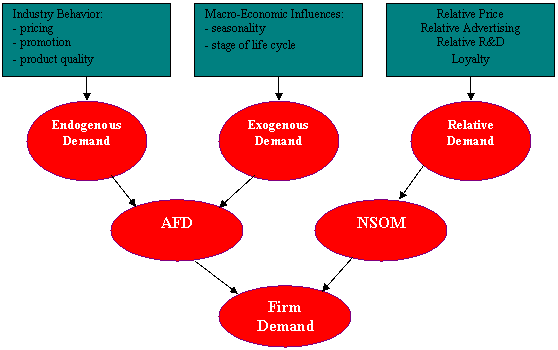
This influence diagram is a graphical representation of the endogenous and exogenous factors that interface with each other to create demand for a product. This diagram will apply tom each of the products the company produced. For this example, demand for each product will be known and not subject to outside or inside factors. This model will give the reader a better example of real life situations.

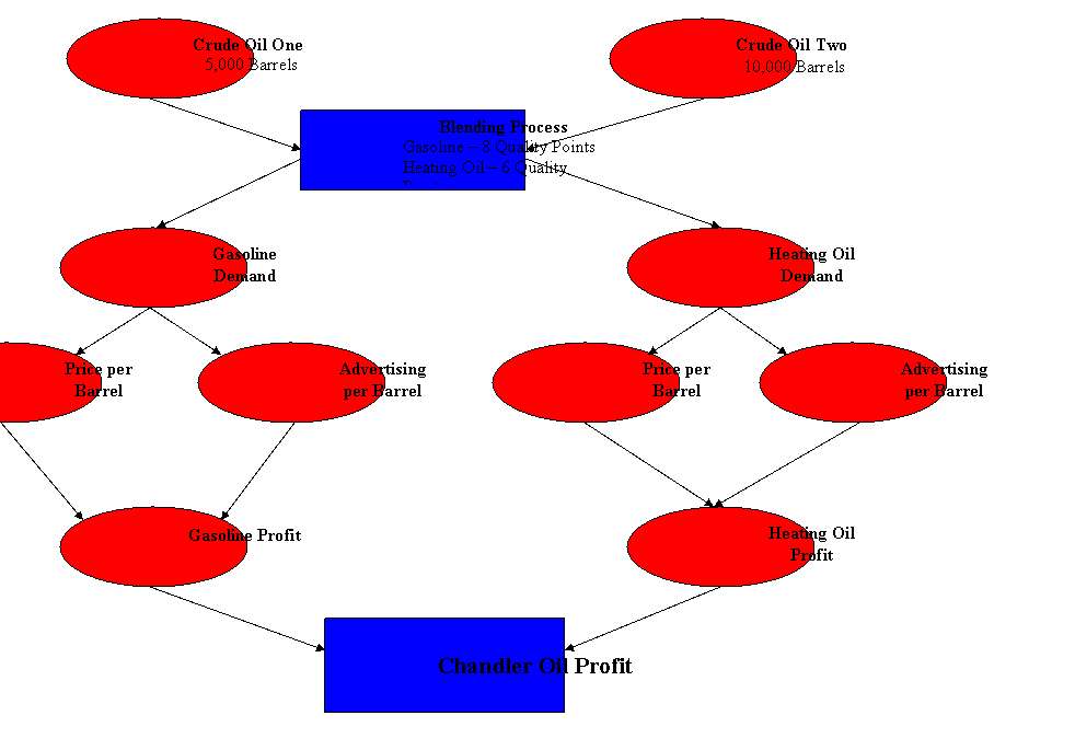
Profit Diagram

Mathematical Representation
|
Blending Combinations
– Will be calculated using excel solver
Gasoline – Minimum three parts crude oil one to two parts crude oil two
Heating Oil – Minimum two parts crude oil one to eight parts crude oil two.
Blending Constraint – To produce the gasoline and the heating oil, a minimum quality level must be obtained. In order to maintain the minimum quality level, the constraint function in the solver will be used. In the constraint function, the minimum quality level will be entered and the solver will not allow the quality level to drop below the constraint entered. Solver will determine the optimal level of production for gasoline and heating oil.
Advertising Cost
Gasoline – Barrels of gasoline produced times $.20
Heating Oil – Barrels of heating oil produce times $0.10
Revenue
Gasoline – Barrels of gasoline produced times $25
Heating Oil – Barrels of gasoline produced times $20
Profit – Will be calculated
using excel solver
(Barrels of gasoline produced times the selling price per barrel) minus (barrels of gasoline produced times advertising cost per barrel) plus
(Barrels of heating oil produced times the selling price per barrel) minus ( barrels of heating oil produced times the advertising price per barrel)
Objective – maximizing profit is the overall objective of this example. Solver will compute the maximum profit taking all of the constraints into consideration. In this model, price and advertising are fixed, therefore solver will change the blending plan for production of gasoline and heating oil to find the maximum profit.
Solver will determine the optimal profit level at the given variables and constraints. The parameters for the solver are shown in the picture below.
|
Development of Spreadsheet Model and Results |
The following snapshot represents the model built using Microsoft Excel
In order to use optimization, the model must contain the following:
- Inputs
- Selling Price – Market Price for Each Product
- Advertising – Expenditure for Each Product
- Barrels Available – Barrels available for production
- Oil Quality Level – Given by quality of resources.
- Blending Plan – Calculated using solver based on quality constraints
- Profit – Objective of model given all inputs and constraints
The following is the results from the model. The figures in the red box represent the blending plan computed using solver. Using the given inputs, the maximum profit level occurs when Chandler Oil produces 5,000 barrels of gasoline and 10,000 barrels of heating oil.
|
|
|
|
|
|
||
|
|
|
|
|
|
|
|
|
Monetary
inputs |
Gasoline |
Heating oil |
|
|
|
|
|
Selling
price/barrel |
$20.00 |
|
|
|
||
|
Advertising
cost/barrel |
$0.10 |
|
|
|
||
|
|
|
|
|
|
|
|
|
Quality
level per barrel of crude oil |
|
|
|
|
||
|
Crude oil
1 |
|
|
|
|
||
|
Crude oil
2 |
5 |
|
|
|
|
|
|
|
|
|
|
|
|
|
|
Required
quality level per barrel of product |
|
|
|
|||
|
|
Gasoline |
Heating oil |
|
|
|
|
|
|
8 |
6 |
|
|
|
|
|
|
|
|
|
|
|
|
|
Blending
plan (barrels of crude in each product) |
|
|
|
|||
|
|
Gasoline |
Heating oil |
Barrels used |
|
Barrels available |
|
|
Crude oil
1 |
2000 |
<= |
||||
|
Crude oil
2 |
2000 |
8000 |
10000 |
<= |
10000 |
|
|
Barrels
sold |
10000 |
|
|
|
||
|
|
|
|
|
|
|
|
|
Constraints
on quality |
|
|
|
|
|
|
|
|
Gasoline |
Heating oil |
|
|
|
|
|
Quality
"points" obtained |
60000 |
|
|
|
||
|
|
>= |
>= |
|
|
|
|
|
Quality
"points" required |
60000 |
|
|
|
||
|
|
|
|
|
|
|
|
|
Monetary
summary |
|
|
|
|
|
|
|
Revenue |
|
|
|
|
||
|
Advertising
cost |
|
|
|
|
||
|
Profit |
|
|
|
|
||
Sensitivity Analysis
The selling price and availability of crude oil one can be changed to determine the optimal profit level. The examples below show how the profit level will change by changing the variables.
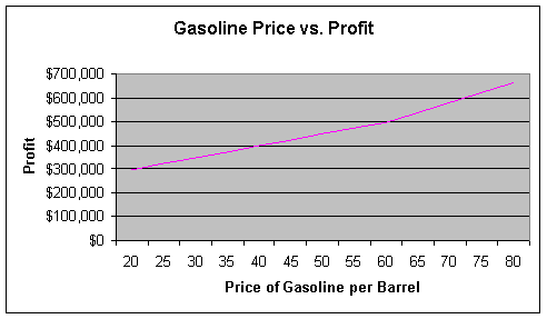
The first example shows how a change in price will affect the change in profit. Looking at the example, with price starting at $20 and increasing at $5 increments, one can see the additional profit earned by the price change. As the price of gasoline increases, the production level of gasoline will increase and the production of heating oil will be reduced to find the optimal profit level at given price levels.
|
Sensitivity
of profit and outputs sold to the selling price of gasoline |
||||
|
Price of gasoline |
Gasoline |
Heating oil |
Profit |
|
|
|
$B$19 |
$C$19 |
$B$30 |
Increase |
|
20 |
0 |
15000 |
$298,500 |
|
|
25 |
5000 |
10000 |
$323,000 |
$24,500 |
|
30 |
5000 |
10000 |
$348,000 |
$25,000 |
|
35 |
5000 |
10000 |
$373,000 |
$25,000 |
|
40 |
5000 |
10000 |
$398,000 |
$25,000 |
|
45 |
5000 |
10000 |
$423,000 |
$25,000 |
|
50 |
5000 |
10000 |
$448,000 |
$25,000 |
|
55 |
5000 |
10000 |
$473,000 |
$25,000 |
|
60 |
8333 |
0 |
$498,333 |
$25,333 |
|
65 |
8333 |
0 |
$540,000 |
$41,667 |
|
70 |
8333 |
0 |
$581,667 |
$41,667 |
|
75 |
8333 |
0 |
$623,333 |
$41,667 |
|
80 |
8333 |
0 |
$665,000 |
$41,667 |

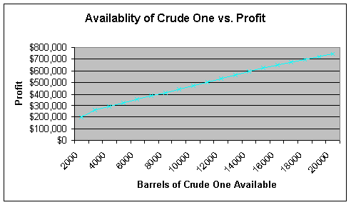
The following chart represents the change in profit based on the availability of crude oil one. Since crude oil one has higher quality content, as the quantity available increases, more gasoline will be produced maximizing profits. An important issue to remember in this model is that cost of the raw materials and the cost to produce the product is not considered. This is mostly a revenue model.
|
Sensitivity
of profit and outputs sold to the availability of crude 1 |
|
|||
|
Availability of crude 1 |
Gasoline |
Heating oil |
Profit |
|
|
|
$B$19 |
$C$19 |
$B$30 |
Increase |
|
2000 |
0 |
10000 |
$199,000 |
|
|
3000 |
1000 |
12000 |
$263,600 |
$64,600 |
|
4000 |
3000 |
11000 |
$293,300 |
$29,700 |
|
5000 |
5000 |
10000 |
$323,000 |
$29,700 |
|
6000 |
7000 |
9000 |
$352,700 |
$29,700 |
|
7000 |
9000 |
8000 |
$382,400 |
$29,700 |
|
8000 |
11000 |
7000 |
$412,100 |
$29,700 |
|
9000 |
13000 |
6000 |
$441,800 |
$29,700 |
|
10000 |
15000 |
5000 |
$471,500 |
$29,700 |
|
11000 |
17000 |
4000 |
$501,200 |
$29,700 |
|
12000 |
19000 |
3000 |
$530,900 |
$29,700 |
|
13000 |
21000 |
2000 |
$560,600 |
$29,700 |
|
14000 |
23000 |
1000 |
$590,300 |
$29,700 |
|
15000 |
25000 |
0 |
$620,000 |
$29,700 |
|
16000 |
26000 |
0 |
$644,800 |
$24,800 |
|
17000 |
27000 |
0 |
$669,600 |
$24,800 |
|
18000 |
28000 |
0 |
$694,400 |
$24,800 |
|
19000 |
29000 |
0 |
$719,200 |
$24,800 |
|
20000 |
30000 |
0 |
$744,000 |
$24,800 |

To test the model, and to view the behind the scenes calculations and results, go to the following link:
When viewing the spreadsheet try changing the some of the inputs to see how those changes will change profit levels. In order to use solver, in the spreadsheet go to the tools function at the top of the spreadsheet. Then press the solve button and see the changed results.
DSS Guidelines
|
This model could be used in a much larger model that incorporates the firm’s entire operations. Optimization can find the optimal level taking into account all of the variables and constraints that a company might have. By changing the inputs or variables in all of the company’s’ functions, the user could see not only the outcome of demand and production, but also what affect this would have on the firm’s financial statements.
Analyses could be conducted to answer any questions about how much to spend on advertising and expenditures, what to price the product to get the desired market share and resulting revenue. This would be an example of goal-seeking where the desired output is entered and the variables are found that create that result. This module could also be used to evaluate scenarios such as good economy or recession. And it could be used to run what-if analyses, for example to see the result in a big increase in advertising will have on product demand.